Measuring variation

The Quality Toolbook > Variation > Measuring variation

Distribution of results | The Central Limit Theorem | Measuring distribution

<-- Previous | Next -->

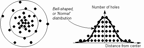
Variation is not simple to measure, as by its nature is random and individual events cannot be predicted. Despite this, a degree of measurement can be achieved by looking at how a number of measurements group together. Usually these items are selected with sampling methods.

The spread of measurements within a group enables special causes of variation to be distinguished from common causes of variation. Beyond this, the characteristics of how these random events are spread out can allow improvements in seemingly random chaos to be simply measured.

Distribution of results

It is common in processes for most measurements to cluster around a central value, with less and less measurements occurring further away from this center. For example, the distribution of holes across the target will gradually spread out from a central, most common placement, as below:

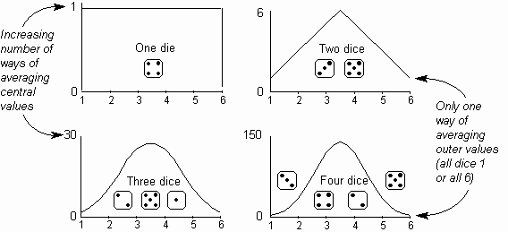
The Normal distribution

The bell-shaped curve in the figure above occurs surprisingly often and is consequently called a Normal distribution (or Gaussian distribution, after its discoverer) and has some very useful properties which can be used to help variation be understood and controlled.

Other distributions

A Normal distribution of measurement values does not always occur, and other distributions may be caused by various factors, conditions and combinations. Several of these are discussed in Chapter 23. It is a trap to use tools that expect a Normal distribution, such as Process Capability, when the distribution is not Normal.

The Central Limit Theorem

The reason for the common occurrence of this Normal distribution is either a natural distribution or the very useful and remarkable effect described by the Central Limit Theorem. This states that, even where the underlying population distribution is not normal, the distribution of the averages of a set of samples will be approximately normal.

This is clearly illustrated below, which shows the distribution of average values achieved by throwing all possible combinations of one, two, three and four dice.

With a single die, the distribution is rectangular, as there is one, equally likely way of achieving each number. With two dice, the distribution becomes triangular, as although there is only one way of averaging one (two ones), there are six ways of averaging the central value of 3.5 (1-6, 2-5, 3-4, 4-3, 5-2 and 6-1).

With three dice, the distribution becomes curved, and with four dice it is markedly bell-shaped, as there is still only one way of averaging one, but there are four ways of averaging 1.25 (three 1s and a 2) and so on up to 147 ways of averaging 3.5! A key use of this effect is that a predictable Normal distribution can be produced by measuring samples in groups of as few as four items at a time.

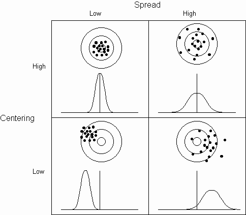
Measuring distribution

The measurements of a process can vary in two different ways, in terms of their centering and their spread, as illustrated below:

The centering (also called accuracy or central tendency) of a process, is the degree to which measurements gather around a target value. The spread (also called dispersion or precision) of the process is the degree of scatter of its output values.

<-- Previous | Next -->